
Differential Expression (DE) analysis is a foundational technique in the field of transcriptomics, allowing researchers to identify genes that exhibit significant changes in expression between two or more biological conditions. Whether exploring the genetic basis of diseases, assessing drug response, or understanding fundamental cellular processes, DE analysis using RNA sequencing (RNA-seq) data provides a high-resolution snapshot of gene activity. This article offers a comprehensive look at DE analysis—from data preprocessing to advanced tools, statistical modeling, and best practices for achieving accurate, reproducible results.
What Is Differential Expression (DE) Analysis?
DE analysis aims to pinpoint genes that show statistically significant differences in expression across distinct experimental groups, such as treated vs. control, or healthy vs. diseased samples. Unlike microarrays, RNA-seq quantifies gene expression through read counts, enabling unbiased, genome-wide profiling with higher sensitivity and specificity.
Why Is DE Analysis Important?
By identifying differentially expressed genes (DEGs), scientists can:
– Discover biomarkers for disease detection or prognosis.
– Characterize gene regulation and pathway alterations.
– Evaluate treatment efficacy or toxicity.
– Understand complex traits through gene expression patterns.
These insights can guide therapeutic interventions, inform personalized medicine, and uncover new biological mechanisms.
The DE Analysis Workflow
A typical DE analysis pipeline involves the following steps:
1. Quality Control (QC): Tools like FastQC and MultiQC assess read quality to ensure clean, interpretable data.
2. Read Alignment: RNA-seq reads are mapped to a reference genome using tools such as STAR or HISAT2.
3. Quantification: FeatureCounts or HTSeq-count assign reads to genes, generating a count matrix for downstream analysis.
4. Normalization: DE analysis requires normalization to correct for library size and sequencing depth. Methods include:
– TMM (Trimmed Mean of M-values) in edgeR
– Median-of-ratios in DESeq2
5. Statistical Testing: Count data is modeled using a negative binomial distribution to accommodate overdispersion. Tools compute p-values and adjust for multiple comparisons using false discovery rate (FDR) correction.
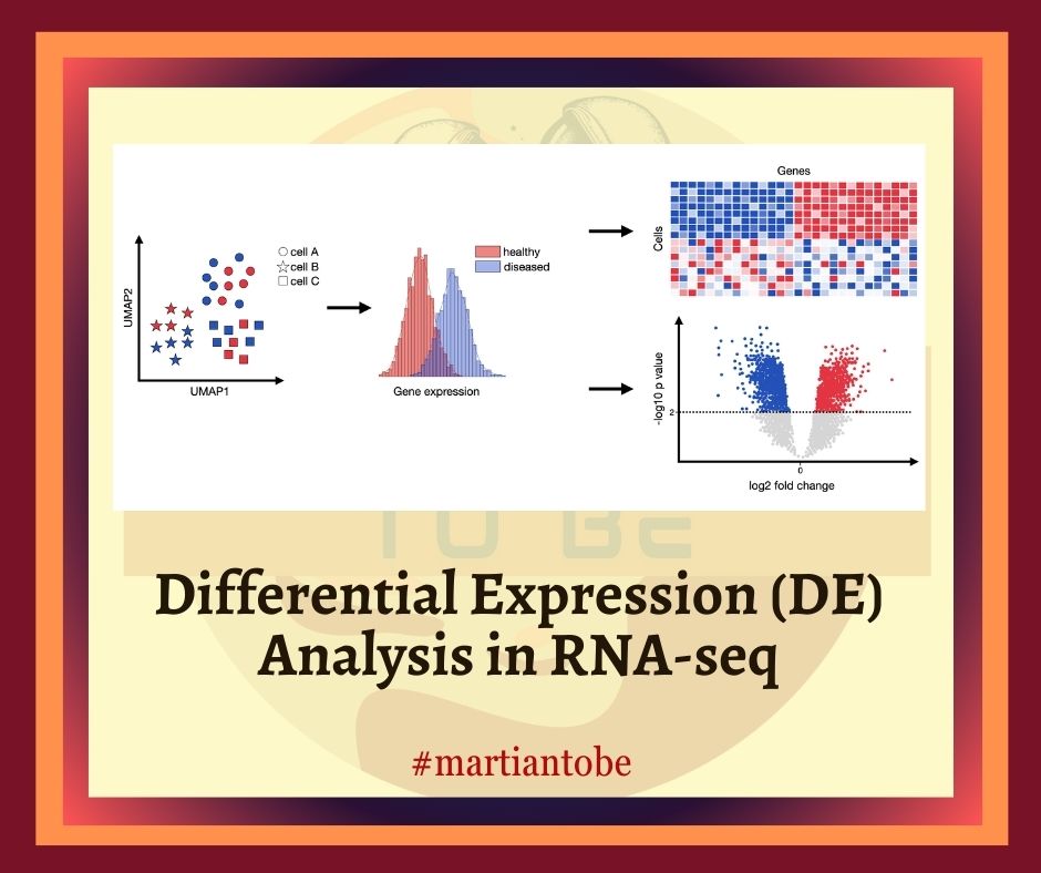
6. Visualization and Interpretation: DEGs are visualized using volcano plots, heatmaps, and PCA plots. Gene Ontology (GO) and pathway enrichment analyses contextualize the biological relevance of findings.
Popular Tools for DE Analysis
Several R/Bioconductor packages are widely used:
– DESeq2: Robust for small sample sizes; uses shrinkage estimators for dispersion and fold change.
– edgeR: Offers flexible modeling and powerful methods for small-sample datasets.
– limma-voom: Combines linear modeling with precision weights; ideal for data with many replicates.
Each tool provides unique strengths—choosing the right one depends on dataset characteristics and research goals.
Handling Batch Effects in DE Analysis
Batch effects—technical variations due to differences in sample handling, sequencing runs, or reagent lots—can confound DE results. Ignoring them can lead to false discoveries or missed DEGs. Modern batch correction methods include:
– ComBat and ComBat-seq: Adjust for additive and multiplicative batch effects using empirical Bayes approaches.
– ComBat-ref: An advanced method that selects a reference batch with minimal dispersion and adjusts others toward it. It preserves count data and significantly improves sensitivity and specificity, especially under severe batch effects.
– NPMatch: A newer, matching-based technique, though it often results in higher false positives compared to ComBat-ref.
Incorporating batch variables into your design matrix or using batch correction prior to DE analysis is essential for trustworthy outcomes.
Best Practices for DE Analysis
To ensure reliable and reproducible results:
– Replicate adequately: Aim for at least 3–5 biological replicates per group.
– Normalize rigorously: Proper normalization is crucial for detecting true biological signals.
– Account for batch effects: Always check for and correct unwanted technical variation.
– Validate findings: Use qPCR, other datasets, or biological replicates for confirmation.
– Document your workflow: Use tools like R Markdown or Snakemake for transparency and reproducibility.
Future Trends in DE Analysis
As single-cell RNA-seq (scRNA-seq) becomes increasingly popular, DE analysis is evolving to address its challenges, such as data sparsity and high dropout rates. Methods like MAST, Seurat, and adaptations of ComBat-ref are being developed to provide accurate DE calls at the single-cell level.
Additionally, machine learning approaches and multi-omics integration are enhancing DE analysis by incorporating more complex biological contexts and covariates.
Differential Expression analysis remains a critical technique for interpreting RNA-seq data, with powerful tools and methods available to uncover meaningful biological insights. By following best practices—especially normalization and batch correction—you can ensure your DE analysis is both accurate and reproducible. As transcriptomics technology advances, DE analysis continues to evolve, offering even more refined and biologically relevant insights into gene regulation and disease mechanisms.
